Note
Go to the end to download the full example code.
Profiling your models
Do you feel like your model is too slow? Do you want to make it faster? Instead of guessing which part of the code is responsible for any slowdown, you should profile your code to learn how much time is spent in each function and where to focus any optimization efforts.
In this tutorial you’ll learn how to profile your model using PyTorch profiler, how to read the output of the profiler, and how to add your own labels for new functions/steps in your model forward function.
from typing import Dict, List, Optional

import ase.build
import matplotlib.pyplot as plt
import numpy as np
import torch

from metatensor.torch import Labels, TensorBlock, TensorMap
from metatensor.torch.atomistic import (
    MetatensorAtomisticModel,
    ModelCapabilities,
    ModelMetadata,
    ModelOutput,
    System,
)
from metatensor.torch.atomistic.ase_calculator import MetatensorCalculator
When profiling your code, it is important to run the model on a representative system to ensure you are actually exercising the behavior of your model at the right scale. Here we’ll use a relatively large system with many atoms.
primitive = ase.build.bulk(name="C", crystalstructure="diamond", a=3.567)
atoms = ase.build.make_supercell(primitive, 10 * np.eye(3))
print(f"We have {len(atoms)} atoms in our system")
We have 2000 atoms in our system
We will use the same HarmonicModel as in the previous tutorial as our machine learning potential.
Click to see the definition of HarmonicModel
class HarmonicModel(torch.nn.Module):
    def __init__(self, force_constant: float, equilibrium_positions: torch.Tensor):
        """Create an ``HarmonicModel``.

        :param force_constant: force constant, in ``energy unit / (length unit)^2``
        :param equilibrium_positions: torch tensor with shape ``n x 3``, containing the
            equilibrium positions of all atoms
        """
        super().__init__()
        assert force_constant > 0
        self.force_constant = force_constant
        self.equilibrium_positions = equilibrium_positions

    def forward(
        self,
        systems: List[System],
        outputs: Dict[str, ModelOutput],
        selected_atoms: Optional[Labels],
    ) -> Dict[str, TensorMap]:
        if list(outputs.keys()) != ["energy"]:
            raise ValueError(
                "this model can only compute 'energy', but `outputs` contains other "
                f"keys: {', '.join(outputs.keys())}"
            )

        # we don't want to worry about selected_atoms yet
        if selected_atoms is not None:
            raise NotImplementedError("selected_atoms is not implemented")

        if outputs["energy"].per_atom:
            raise NotImplementedError("per atom energy is not implemented")

        # compute the energy for each system by adding together the energy for each atom
        energy = torch.zeros((len(systems), 1), dtype=systems[0].positions.dtype)
        for i, system in enumerate(systems):
            assert len(system) == self.equilibrium_positions.shape[0]
            r0 = self.equilibrium_positions
            energy[i] += torch.sum(self.force_constant * (system.positions - r0) ** 2)

        # add metadata to the output
        block = TensorBlock(
            values=energy,
            samples=Labels("system", torch.arange(len(systems)).reshape(-1, 1)),
            components=[],
            properties=Labels("energy", torch.tensor([[0]])),
        )
        return {
            "energy": TensorMap(keys=Labels("_", torch.tensor([[0]])), blocks=[block])
        }


model = HarmonicModel(
    force_constant=3.14159265358979323846,
    equilibrium_positions=torch.tensor(atoms.positions),
)

capabilities = ModelCapabilities(
    outputs={
        "energy": ModelOutput(quantity="energy", unit="eV", per_atom=False),
    },
    atomic_types=[6],
    interaction_range=0.0,
    length_unit="Angstrom",
    supported_devices=["cpu"],
    dtype="float32",
)

metadata = ModelMetadata()
wrapper = MetatensorAtomisticModel(model.eval(), metadata, capabilities)

wrapper.export("exported-model.pt")
/home/runner/work/metatensor/metatensor/python/examples/atomistic/4-profiling.py:128: DeprecationWarning: `export()` is deprecated, use `save()` instead
  wrapper.export("exported-model.pt")
If you are trying to profile your own model, you can start here and create a
MetatensorCalculator with your own model.
atoms.calc = MetatensorCalculator("exported-model.pt")
Before trying to profile the code, it is a good idea to run it a couple of times to allow torch to warmup internally.
atoms.get_forces()
atoms.get_potential_energy()
3.770593615115558e-09
Profiling energy calculation
Now we can run code using torch.profiler.profile() to collect statistic on
how long each function takes to run. We randomize the positions to force ASE to
recompute the energy of the system
atoms.positions += np.random.rand(*atoms.positions.shape)
with torch.profiler.profile() as energy_profiler:
    atoms.get_potential_energy()

print(energy_profiler.key_averages().table(sort_by="self_cpu_time_total", row_limit=10))
--------------------------------------------------  ------------  ------------  ------------  ------------  ------------  ------------
                                              Name    Self CPU %      Self CPU   CPU total %     CPU total  CPU time avg    # of Calls
--------------------------------------------------  ------------  ------------  ------------  ------------  ------------  ------------
                  ASECalculator::compute_neighbors        28.54%     257.491us        28.66%     258.493us     258.493us             1
                     ASECalculator::prepare_inputs        20.38%     183.794us        24.29%     219.150us     219.150us             1
                    ASECalculator::convert_outputs        12.26%     110.567us        13.97%     125.986us      62.993us             2
                                    Model::forward         6.09%      54.903us        18.67%     168.445us     168.445us             1
                                        aten::sort         3.32%      29.975us         5.50%      49.593us      49.593us             1
                                       aten::copy_         3.11%      28.046us         3.11%      28.046us       2.550us            11
                                    aten::_to_copy         2.52%      22.740us         6.07%      54.741us       6.082us             9
                                      aten::arange         2.29%      20.700us         4.56%      41.147us      10.287us             4
                                    aten::_unique2         2.22%      20.046us         8.17%      73.728us      73.728us             1
                                         aten::sum         1.89%      17.050us         1.99%      17.983us      17.983us             1
--------------------------------------------------  ------------  ------------  ------------  ------------  ------------  ------------
Self CPU time total: 902.056us
There are a couple of interesting things to see here. First the total runtime of the
code is shown in the bottom; and then the most costly functions are visible on top,
one line per function. For each function, Self CPU refers to the time spent in
this function excluding any called functions; and CPU total refers to the time
spent in this function, including called functions.
For more options to record operations and display the output, please refer to the official documentation for PyTorch profiler.
Here, Model::forward indicates the time taken by your model’s forward().
Anything starting with aten:: comes from operations on torch tensors, typically
with the same function name as the corresponding torch functions (e.g.
aten::arange is torch.arange()). We can also see some internal functions
from metatensor, with the name staring with MetatensorAtomisticModel:: for
MetatensorAtomisticModel; and ASECalculator:: for
ase_calculator.MetatensorCalculator.
If you want to see more details on the internal steps taken by your model, you can add
torch.profiler.record_function()
(https://pytorch.org/docs/stable/generated/torch.autograd.profiler.record_function.html)
inside your model code to give names to different steps in the calculation. This is
how we are internally adding names such as Model::forward or
ASECalculator::prepare_inputs above.
Profiling forces calculation
Let’s now do the same, but computing the forces for this system. This mean we should
now see some time spent in the backward() function, on top of everything else.
atoms.positions += np.random.rand(*atoms.positions.shape)
with torch.profiler.profile() as forces_profiler:
    atoms.get_forces()

print(forces_profiler.key_averages().table(sort_by="self_cpu_time_total", row_limit=10))
-------------------------------------------------------  ------------  ------------  ------------  ------------  ------------  ------------
                                                   Name    Self CPU %      Self CPU   CPU total %     CPU total  CPU time avg    # of Calls
-------------------------------------------------------  ------------  ------------  ------------  ------------  ------------  ------------
torch::jit::(anonymous namespace)::DifferentiableGra...        32.99%     742.809us        37.04%     833.909us     833.909us             1
                                         Model::forward        15.99%     360.038us        20.35%     458.087us     458.087us             1
                         ASECalculator::convert_outputs         9.54%     214.831us        12.08%     271.898us     135.949us             2
                          ASECalculator::prepare_inputs         9.07%     204.253us        12.99%     292.507us     292.507us             1
                            ASECalculator::run_backward         5.51%     124.123us        48.40%       1.090ms       1.090ms             1
                                               aten::mm         3.74%      84.156us         3.77%      84.908us      21.227us             4
                                            aten::copy_         2.52%      56.816us         2.52%      56.816us       2.706us            21
                                              aten::mul         1.86%      41.898us         2.42%      54.511us      13.628us             4
                       ASECalculator::compute_neighbors         1.67%      37.672us         1.71%      38.603us      38.603us             1
                                          <backward op>         1.62%      36.498us         4.05%      91.100us      91.100us             1
-------------------------------------------------------  ------------  ------------  ------------  ------------  ------------  ------------
Self CPU time total: 2.252ms
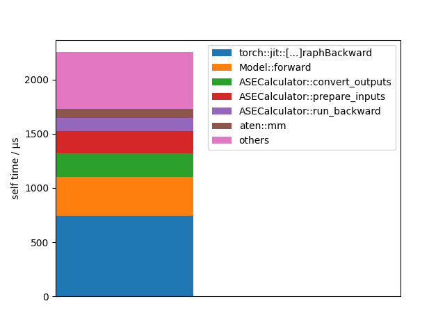
Let’s visualize this data in an other way:
events = forces_profiler.key_averages()
events = sorted(events, key=lambda u: u.self_cpu_time_total, reverse=True)
total_cpu_time = sum(map(lambda u: u.self_cpu_time_total, events))

bottom = 0.0
for event in events:
    self_time = event.self_cpu_time_total
    name = event.key
    if len(name) > 30:
        name = name[:12] + "[...]" + name[-12:]

    if self_time > 0.03 * total_cpu_time:
        plt.bar(0, self_time, bottom=bottom, label=name)
        bottom += self_time
    else:
        plt.bar(0, total_cpu_time - bottom, bottom=bottom, label="others")
        break

plt.legend()
plt.xticks([])
plt.xlim(0, 1)
plt.ylabel("self time / µs")
plt.show()
Total running time of the script: (0 minutes 0.270 seconds)