Note
Go to the end to download the full example code.
Profiling your models
Do you feel like your model is too slow? Do you want to make it faster? Instead of guessing which part of the code is responsible for the slowdown, you should profile your code to learn how much time is spent in each function and where to focus any optimization efforts.
In this tutorial you’ll learn how to profile your model using the PyTorch profiler, how to read the output of the profiler, and how to add your own labels for new functions/steps in your model’s forward function.
from typing import Dict, List, Optional

import ase.build
import matplotlib.pyplot as plt
import numpy as np
import torch
from metatensor.torch import Labels, TensorBlock, TensorMap

from metatomic.torch import (
    AtomisticModel,
    ModelCapabilities,
    ModelMetadata,
    ModelOutput,
    System,
)
from metatomic_ase import MetatomicCalculator
When profiling your code, it is important to run the model on a representative system to ensure you are actually exercising the behavior of your model at the right scale. Here we’ll use a relatively large system with many atoms.
primitive = ase.build.bulk(name="C", crystalstructure="diamond", a=3.567)
atoms = ase.build.make_supercell(primitive, 10 * np.eye(3))
print(f"We have {len(atoms)} atoms in our system")
We have 2000 atoms in our system
We will use the same HarmonicModel as in the previous tutorial as our machine learning potential.
Click to see the definition of HarmonicModel
class HarmonicModel(torch.nn.Module):
    def __init__(self, force_constant: float, equilibrium_positions: torch.Tensor):
        """Create an ``HarmonicModel``.

        :param force_constant: force constant, in ``energy unit / (length unit)^2``
        :param equilibrium_positions: torch tensor with shape ``n x 3``, containing the
            equilibrium positions of all atoms
        """
        super().__init__()
        assert force_constant > 0
        self.force_constant = force_constant
        self.equilibrium_positions = equilibrium_positions

    def forward(
        self,
        systems: List[System],
        outputs: Dict[str, ModelOutput],
        selected_atoms: Optional[Labels],
    ) -> Dict[str, TensorMap]:
        if list(outputs.keys()) != ["energy"]:
            raise ValueError(
                "this model can only compute 'energy', but `outputs` contains other "
                f"keys: {', '.join(outputs.keys())}"
            )

        # we don't want to worry about selected_atoms yet
        if selected_atoms is not None:
            raise NotImplementedError("selected_atoms is not implemented")

        if outputs["energy"].sample_kind == "atom":
            raise NotImplementedError("per atom energy is not implemented")

        # compute the energy for each system by adding together the energy for each atom
        energy = torch.zeros((len(systems), 1), dtype=systems[0].positions.dtype)
        for i, system in enumerate(systems):
            assert len(system) == self.equilibrium_positions.shape[0]
            r0 = self.equilibrium_positions
            energy[i] += torch.sum(self.force_constant * (system.positions - r0) ** 2)

        # add metadata to the output
        block = TensorBlock(
            values=energy,
            samples=Labels("system", torch.arange(len(systems)).reshape(-1, 1)),
            components=[],
            properties=Labels("energy", torch.tensor([[0]])),
        )
        return {
            "energy": TensorMap(keys=Labels("_", torch.tensor([[0]])), blocks=[block])
        }


model = HarmonicModel(
    force_constant=3.14159265358979323846,
    equilibrium_positions=torch.tensor(atoms.positions),
)

capabilities = ModelCapabilities(
    outputs={
        "energy": ModelOutput(unit="eV", sample_kind="system"),
    },
    atomic_types=[6],
    interaction_range=0.0,
    length_unit="Angstrom",
    supported_devices=["cpu"],
    dtype="float32",
)

metadata = ModelMetadata()
wrapper = AtomisticModel(model.eval(), metadata, capabilities)

wrapper.export("exported-model.pt")
/home/runner/work/metatomic/metatomic/python/examples/4-profiling.py:128: DeprecationWarning: `export()` is deprecated, use `save()` instead
  wrapper.export("exported-model.pt")
If you are trying to profile your own model, you can start here and create
MetatomicCalculator with your own model.
Profiling energy calculation
We will start with an energy-only calculator, which can be enabled with
do_gradients_with_energy=False.
atoms.calc = MetatomicCalculator("exported-model.pt", do_gradients_with_energy=False)
Before trying to profile the code, it is a good idea to run it a couple of times to allow torch to warmup internally.
for _ in range(10):
    # force the model to re-run everytime, otherwise ASE caches calculation results
    atoms.rattle(1e-6)
    atoms.get_potential_energy()
Now we can run code using torch.profiler.profile() to collect statistic on
how long each function takes to run.
atoms.rattle(1e-6)
with torch.profiler.profile() as energy_profiler:
    atoms.get_potential_energy()

print(energy_profiler.key_averages().table(sort_by="self_cpu_time_total", row_limit=10))
------------------------------------------  ------------  ------------  ------------  ------------  ------------  ------------
                                      Name    Self CPU %      Self CPU   CPU total %     CPU total  CPU time avg    # of Calls
------------------------------------------  ------------  ------------  ------------  ------------  ------------  ------------
       MetatomicCalculator::prepare_inputs        19.67%     212.662us        26.63%     287.803us     287.803us             1
    MetatomicCalculator::compute_neighbors         9.54%     103.073us        16.21%     175.168us     175.168us             1
                            Model::forward         7.65%      82.691us        19.04%     205.772us     205.772us             1
       AtomisticModel::convert_units_input         7.16%      77.415us        11.22%     121.238us     121.238us             1
         MetatomicCalculator::sum_energies         6.86%      74.169us         6.86%      74.169us      74.169us             1
        AtomisticModel::check_atomic_types         4.49%      48.581us         9.06%      97.974us      97.974us             1
      AtomisticModel::convert_units_output         4.43%      47.841us         4.63%      50.034us      50.034us             1
                                   forward         3.81%      41.179us        11.39%     123.081us     123.081us             1
      MetatomicCalculator::convert_outputs         2.97%      32.089us         4.25%      45.948us      45.948us             1
                            aten::_to_copy         2.46%      26.559us         6.36%      68.790us       4.299us            16
------------------------------------------  ------------  ------------  ------------  ------------  ------------  ------------
Self CPU time total: 1.081ms
There are a couple of interesting things to see here. First the total runtime of the
code is shown in the bottom; and then the most costly functions are visible on top,
one line per function. For each function, Self CPU refers to the time spent in
this function excluding any called functions; and CPU total refers to the time
spent in this function, including called functions.
For more options to record operations and display outputs, please refer to the official documentation for PyTorch profiler.
Here, Model::forward indicates the time taken by your model’s forward().
Anything starting with aten:: comes from operations on torch tensors, typically
with the same function name as the corresponding torch functions (e.g.
aten::arange is torch.arange()). We can also see some internal functions
from metatomic, with the name staring with AtomisticModel:: for
AtomisticModel; and MetatomicCalculator:: for
ase_calculator.MetatomicCalculator.
If you want to see more details on the internal steps taken by your model, you
can add torch.profiler.record_function()
(https://pytorch.org/docs/stable/generated/torch.autograd.profiler.record_function.html)
inside your model code to give names to different steps in the calculation.
This is how we internally set names such as Model::forward or
MetatomicCalculator::prepare_inputs above.
Profiling forces calculation
Let us now do the same, but while also computing the forces for this system.
This mean we should now see some time spent in the backward() function, on
top of everything else.
atoms.calc = MetatomicCalculator("exported-model.pt")

# warmup
for _ in range(10):
    atoms.rattle(1e-6)
    atoms.get_forces()

atoms.rattle(1e-6)
with torch.profiler.profile() as forces_profiler:
    atoms.get_forces()

print(forces_profiler.key_averages().table(sort_by="self_cpu_time_total", row_limit=10))
-------------------------------------------------------  ------------  ------------  ------------  ------------  ------------  ------------
                                                   Name    Self CPU %      Self CPU   CPU total %     CPU total  CPU time avg    # of Calls
-------------------------------------------------------  ------------  ------------  ------------  ------------  ------------  ------------
                    MetatomicCalculator::prepare_inputs        15.08%     232.470us        21.90%     337.556us     337.556us             1
                      MetatomicCalculator::run_backward         7.89%     121.609us        20.06%     309.224us     309.224us             1
                   MetatomicCalculator::convert_outputs         7.21%     111.105us         9.69%     149.370us     149.370us             1
                 MetatomicCalculator::compute_neighbors         6.97%     107.490us        12.24%     188.668us     188.668us             1
                                         Model::forward         5.76%      88.730us        14.64%     225.581us     225.581us             1
                    AtomisticModel::convert_units_input         5.16%      79.526us         8.27%     127.527us     127.527us             1
                                               aten::mm         4.49%      69.169us         4.55%      70.122us      17.531us             4
                                                forward         3.50%      53.929us         8.88%     136.851us     136.851us             1
                   AtomisticModel::convert_units_output         3.21%      49.443us         3.35%      51.566us      51.566us             1
                                            aten::copy_         2.96%      45.559us         2.96%      45.559us       1.687us            27
-------------------------------------------------------  ------------  ------------  ------------  ------------  ------------  ------------
Self CPU time total: 1.541ms
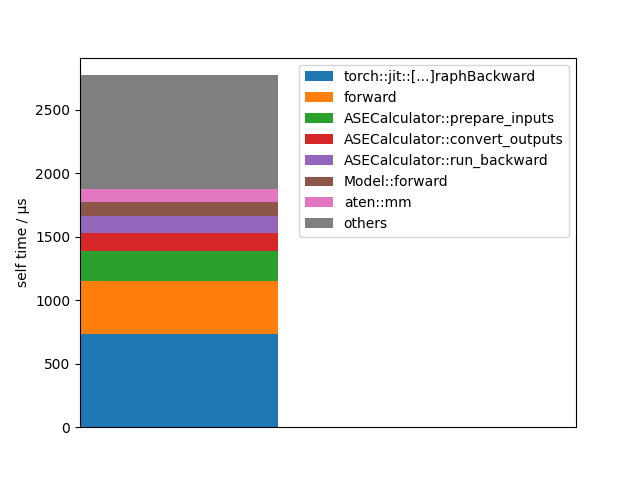
Let’s visualize this data in another way:
events = forces_profiler.key_averages()
events = sorted(events, key=lambda u: u.self_cpu_time_total, reverse=True)
total_cpu_time = sum(map(lambda u: u.self_cpu_time_total, events))

bottom = 0.0
for event in events:
    self_time = event.self_cpu_time_total
    name = event.key
    if len(name) > 30:
        name = name[:12] + "[...]" + name[-12:]

    if self_time > 0.03 * total_cpu_time:
        plt.bar(0, self_time, bottom=bottom, label=name)
        bottom += self_time
    else:
        plt.bar(0, total_cpu_time - bottom, bottom=bottom, label="others")
        break

plt.legend()
plt.xticks([])
plt.xlim(0, 1)
plt.ylabel("self time / µs")
plt.show()
Total running time of the script: (0 minutes 0.272 seconds)