Fine-tuning a pre-trained model

This is a simple example for fine-tuning PET-MAD (or a general PET model), that can be used as a template for general fine-tuning with metatrain. Fine-tuning a pretrained model allows you to obtain a model better suited for your specific system. You need a dataset of structures with reference energies and forces for the task you want to model. Fine-tuning uses a pretrained checkpoint with the mtt train command and the options-ft.yaml file. The reference data can use the same level of theory as the pretrained model or a different one.

We start by setting up the options-ft.yaml file. Here we specify to fine-tune on a small dataset containing structures of ethanol, labelled with energies and forces. We can specify the fine-tuning method in the finetune block in the training options of the architecture. Here, the basic full option is chosen, which finetunes all weights of the model. All available fine-tuning methods are found in the concepts page Fine-tuning. This section discusses implementation details, options and recommended use cases. Other fine-tuning options can be simply substituted in this script, by changing the finetune block.

Note

This example creates a new energy head by requesting the target energy/finetune. To choose another name, use energy/{yourname}.

Furthermore, you need to specify the checkpoint, that you want to fine-tune in the read_from option.

A simple options-ft.yaml file for this task could look like this:

architecture:
  name: pet
  training:
    batch_size: 8
    num_epochs: 10
    learning_rate: 1e-3
    warmup_fraction: 0.01
    finetune:
      method: full
      read_from: pet-mad-v1.1.0.ckpt

training_set:
  systems:
    read_from: ethanol_reduced_100.xyz
    reader: ase
    length_unit: angstrom
  targets:
    energy/finetune:
      quantity: energy
      read_from: ethanol_reduced_100.xyz
      reader: ase
      key: energy
      unit: eV
      description: pbe energy ethanol
      forces:
        read_from: ethanol_reduced_100.xyz
        reader: ase
        key: forces

validation_set: 0.1
test_set: 0.1

This example uses only ten epochs and a learning rate of 1e-3 to keep the demonstration short. For your own task, start with a learning rate lower than the original training run and use validation performance to choose how long to train.

This example creates an energy/finetune target with its own head and composition baseline. Since we use full fine-tuning and do not train the original energy target, that original target is removed.

We fine-tune the pretrained model on ethanol_reduced_100.xyz, which stores reference energies under energy and forces under forces. The targets section of options-ft.yaml maps these keys to the energy/finetune target. Further information on specifying targets can be found in the data section of the Training YAML Reference.

Note

Set length_unit and the target unit to match your reference data. This dataset uses angstrom and eV.

After setting up your options-ft.yaml file, you can then simply run:

mtt train options-ft.yaml -o model-ft.pt

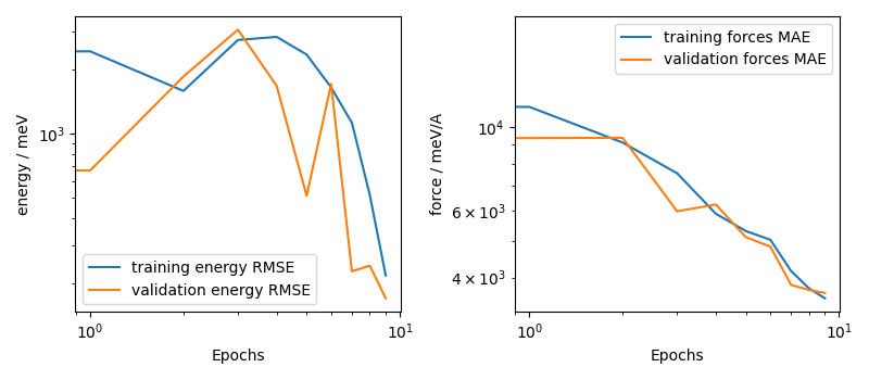
You can check fine-tuning training curves by parsing the train.csv written by mtt train.

import glob
import subprocess

import ase.io
import matplotlib.pyplot as plt
import numpy as np
from metatomic_ase import MetatomicCalculator

# In order to obtain a pretrained model, you can use a PET-MAD checkpoint from
# Hugging Face. Here, we download the checkpoint and run ``mtt train`` as a subprocess.

subprocess.run(
    [
        "wget",
        "https://huggingface.co/lab-cosmo/pet-mad/resolve/v1.1.0/models/pet-mad-v1.1.0.ckpt",
    ],
    check=True,
)

subprocess.run(["mtt", "train", "options-ft.yaml", "-o", "model-ft.pt"], check=True)

CompletedProcess(args=['mtt', 'train', 'options-ft.yaml', '-o', 'model-ft.pt'], returncode=0)

After training, we inspect the learning curves saved in train.csv. We select the latest run from the date and time-stamped outputs folders.

csv_path = sorted(glob.glob("outputs/*/*/train.csv"))[-1]
with open(csv_path, "r") as f:
    header = f.readline().strip().split(",")
    f.readline()  # skip units row

# Build dtype
dtype = [(h, float) for h in header]

# Load data as plain float array
data = np.loadtxt(csv_path, delimiter=",", skiprows=2, ndmin=2)

# Convert to structured
structured = np.zeros(data.shape[0], dtype=dtype)
for i, h in enumerate(header):
    structured[h] = data[:, i]

Now, let’s plot the learning curves.

epochs = structured["Epoch"]
training_energy_RMSE = structured["training energy/finetune RMSE (per atom)"]
training_forces_MAE = structured["training forces[energy/finetune] MAE"]
validation_energy_RMSE = structured["validation energy/finetune RMSE (per atom)"]
validation_forces_MAE = structured["validation forces[energy/finetune] MAE"]

fig, axs = plt.subplots(1, 2, figsize=((8, 3.5)))

axs[0].plot(epochs, training_energy_RMSE, label="training energy RMSE")
axs[0].plot(epochs, validation_energy_RMSE, label="validation energy RMSE")
axs[0].set_xlabel("Epochs")
axs[0].set_ylabel("Energy RMSE / (meV/atom)")
axs[0].set_yscale("log")
axs[0].legend()
axs[1].plot(epochs, training_forces_MAE, label="training forces MAE")
axs[1].plot(epochs, validation_forces_MAE, label="validation forces MAE")
axs[1].set_ylabel("Force MAE / (meV/Å)")
axs[1].set_xlabel("Epochs")
axs[1].set_yscale("log")
axs[1].legend()
plt.tight_layout()
plt.show()

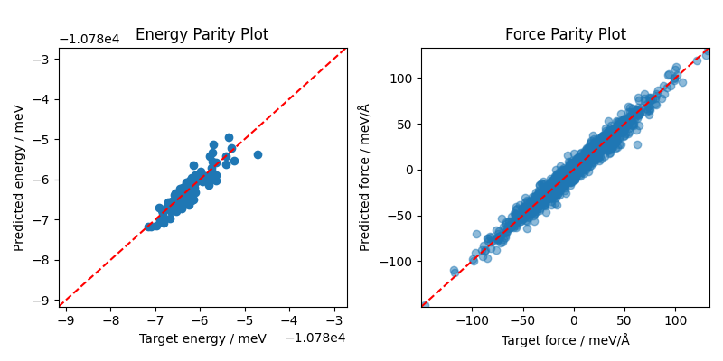
To evaluate the fine-tuned model, we can inspect parity plots for energy and force (see Model validation with parity plots). With mtt eval, specify the new target in options-ft-eval.yaml:

systems: ethanol_reduced_100.xyz
targets:
  energy/finetune:
    key: energy
    unit: eV
    forces:
      key: forces

and then run

mtt eval model-ft.pt options-ft-eval.yaml -o output-ft.xyz

This evaluates the whole example dataset, including training structures. Use a separate held-out dataset to assess generalization. The predicted energies are stored in the headers of the output xyz file. Another possibility is to load your fine-tuned model model-ft.pt as metatomic model and evaluate energies and forces with ASE in Python.

Using the fine-tuned model with ASE

When using a fine-tuned model with ASE, you need to specify which variant to use. Since we trained with the energy/finetune variant, we pass variants={"energy": "finetune"} to the MetatomicCalculator. This tells the calculator to use the fine-tuned energy head instead of the default energy head.

If you fine-tuned with a different variant name (e.g., energy/pbe), you would use variants={"energy": "pbe"} instead.

For LAMMPS simulations, you would specify the variant in your LAMMPS input script:

pair_style metatomic model-ft.pt [...other arguments...] variant finetune

More details on using variants in simulation engines can be found in the metatomic ASE documentation and metatomic LAMMPS documentation.

sphinx_gallery_capture_repr_block = ()

np.seterr()
targets = ase.io.read(
    "ethanol_reduced_100.xyz",
    format="extxyz",
    index=":",
)
calc_ft = MetatomicCalculator(
    "model-ft.pt", variants={"energy": "finetune"}, extensions_directory=None
)
with np.errstate(invalid="ignore"):
    e_targets = np.array(
        [frame.get_potential_energy() / len(frame) for frame in targets]
    )  # target energies
    f_targets = np.array(
        [frame.get_forces().flatten() for frame in targets]
    ).flatten()  # target forces

    for frame in targets:
        frame.calc = calc_ft

    e_predictions = np.array(
        [frame.get_potential_energy() / len(frame) for frame in targets]
    )  # predicted energies
    f_predictions = np.array(
        [frame.get_forces().flatten() for frame in targets]
    ).flatten()  # predicted forces

fig, axs = plt.subplots(1, 2, figsize=(8, 4))

# Parity plot for energies
axs[0].scatter(e_targets, e_predictions, label="FT")
axs[0].axline((np.min(e_targets), np.min(e_targets)), slope=1, ls="--", color="red")
axs[0].set_xlabel("Target energy / eV/atom")
axs[0].set_ylabel("Predicted energy / eV/atom")
min_e = np.min(np.array([e_targets, e_predictions])) - 2
max_e = np.max(np.array([e_targets, e_predictions])) + 2
axs[0].set_title("Energy Parity Plot")
axs[0].set_xlim(min_e, max_e)
axs[0].set_ylim(min_e, max_e)

# Parity plot for forces
axs[1].scatter(f_targets, f_predictions, alpha=0.5, label="FT")
axs[1].axline((np.min(f_targets), np.min(f_targets)), slope=1, ls="--", color="red")
axs[1].set_xlabel("Target force / eV/Å")
axs[1].set_ylabel("Predicted force / eV/Å")
min_f = np.min(np.array([f_targets, f_predictions])) - 2
max_f = np.max(np.array([f_targets, f_predictions])) + 2
axs[1].set_title("Force Parity Plot")
axs[1].set_xlim(min_f, max_f)
axs[1].set_ylim(min_f, max_f)
fig.tight_layout()
plt.show()

/home/runner/work/metatrain/metatrain/.tox/docs/lib/python3.14/site-packages/torch/jit/_serialization.py:170: FutureWarning: `torch.jit.load` is not supported in Python 3.14+ and may break. Please switch to `torch.export`.
  warnings.warn(

Use validation performance to decide whether to train longer or adjust the fine-tuning settings.

Note

To learn about more elaborate fine-tuning strategies and tools, check out the fine-tuning examples in the AtomisticCookbook