Training a Classifier Model

This tutorial demonstrates how to train a classifier model using metatrain. The classifier model is a transfer learning architecture that takes a pre-trained model, freezes its backbone, and trains a small multi-layer perceptron (MLP) on top of the extracted features for classification tasks.

In this example, we will classify carbon allotropes (diamond, graphite, and graphene).

Creating the Dataset

First, we need to create a dataset with different carbon structures. We’ll generate simple structures for diamond, graphite, and graphene, and label them with one-hot encoded class labels. The classifier also supports soft/fractional targets for cases where the class membership is uncertain.

import subprocess

import ase.io
import chemiscope
import matplotlib.pyplot as plt
import numpy as np
from ase.build import bulk, graphene
from metatomic.torch import ModelOutput
from metatomic.torch.ase_calculator import MetatomicCalculator

Helper function to convert class labels to one-hot encodings

This function converts string class labels (e.g., “diamond”, “graphite”, “graphene”) into one-hot encoded probability vectors that the classifier can use for training. You can use it yourself to prepare datasets if you’re starting from string labels.

def class_to_onehot(class_label: str, class_names: list[str]) -> list[float]:
    """Convert a class label string to a one-hot encoded probability vector.

    :param class_label: The class label as a string (e.g., "diamond")
    :param class_names: List of all possible class names in order
    :return: One-hot encoded probability vector (e.g., [1.0, 0.0, 0.0])
    """
    if class_label not in class_names:
        raise ValueError(f"Unknown class label: {class_label}")

    onehot = [0.0] * len(class_names)
    onehot[class_names.index(class_label)] = 1.0
    return onehot

We generate structures for three carbon allotropes:

• Diamond (class 0)

• Graphite (class 1)

• Graphene (class 2)

np.random.seed(42)

# Define class names for the classifier
class_names = ["diamond", "graphite", "graphene"]

structures = []

# Generate 10 diamond structures with small random perturbations
for i in range(10):
    diamond = bulk("C", "diamond", a=3.57)
    diamond = diamond * (2, 2, 2)  # Make it bigger
    diamond.rattle(stdev=0.5, seed=i)  # Add random perturbations
    # Store string label in info, then convert to one-hot
    diamond.info["class_label"] = "diamond"
    diamond.info["class"] = class_to_onehot("diamond", class_names)
    structures.append(diamond)

# Generate 10 graphite structures (using layered graphene-like structures)
for i in range(10):
    # Create a graphite-like structure
    graphite = graphene(formula="C2", size=(3, 3, 1), a=2.46, vacuum=None)
    # Stack two layers
    layer2 = graphite.copy()
    layer2.translate([0, 0, 3.35])
    graphite.extend(layer2)
    graphite.set_cell([graphite.cell[0], graphite.cell[1], [0, 0, 6.7]])
    graphite.rattle(stdev=0.5, seed=i)
    # Store string label in info, then convert to one-hot
    graphite.info["class_label"] = "graphite"
    graphite.info["class"] = class_to_onehot("graphite", class_names)
    structures.append(graphite)

# Generate 10 graphene structures (single layer)
for i in range(10):
    graphene_struct = graphene(formula="C2", size=(3, 3, 1), a=2.46, vacuum=10.0)
    graphene_struct.rattle(stdev=0.5, seed=i)
    # Store string label in info, then convert to one-hot
    graphene_struct.info["class_label"] = "graphene"
    graphene_struct.info["class"] = class_to_onehot("graphene", class_names)
    structures.append(graphene_struct)

# Save the structures to a file (these will be used for training)
ase.io.write("carbon_allotropes.xyz", structures)

Getting a pre-trained universal model

Here, we download a pre-trained model checkpoint that will serve as the backbone for our classifier. We will use PET-MAD, a universal interatomic potential for materials and molecules.

PET_MAD_URL = (
    "https://huggingface.co/lab-cosmo/pet-mad/resolve/v1.0.2/models/pet-mad-v1.0.2.ckpt"
)

subprocess.run(["wget", PET_MAD_URL], check=True)

CompletedProcess(args=['wget', 'https://huggingface.co/lab-cosmo/pet-mad/resolve/v1.0.2/models/pet-mad-v1.0.2.ckpt'], returncode=0)

Training the Classifier

Now we can train the classifier. The classifier will learn to use the features learned by PET-MAD to classify our carbon allotropes.

The key hyperparameters are:

• hidden_sizes: The dimensions of the MLP layers. The last dimension (2 in this case) acts as a bottleneck that can be used to extract collective variables. If collective variables are not needed, this should be set to a larger value.

• model_checkpoint: Path to the pre-trained model (here PET-MAD).

seed: 42

architecture:
  name: experimental.classifier
  model:
    hidden_sizes: [64, 2, 64]
    feature_layer_index: 2
  training:
    model_checkpoint: pet-mad-v1.0.2.ckpt
    num_epochs: 10
    learning_rate: 1e-3
    batch_size: 6
    log_interval: 1

training_set:
  systems:
    read_from: carbon_allotropes.xyz
    length_unit: angstrom
  targets:
    mtt::class_probabilities:
      key: class
      num_subtargets: 3

validation_set: 0.2
test_set: 0.0

# Here, we run training as a subprocess, in reality you would run this from the command
# line as ``mtt train options-classifier.yaml -o classifier.pt``.
subprocess.run(
    ["mtt", "train", "options-classifier.yaml", "-o", "classifier.pt"],
    check=True,
)

CompletedProcess(args=['mtt', 'train', 'options-classifier.yaml', '-o', 'classifier.pt'], returncode=0)

Using the Trained Classifier

Once the classifier is trained, we can use it to predict class labels for new structures or to extract bottleneck features (collective variables).

Let’s test the classifier on some structures:

# Load the model
calc = MetatomicCalculator("classifier.pt")

structures = ase.io.read("carbon_allotropes.xyz", index=":")

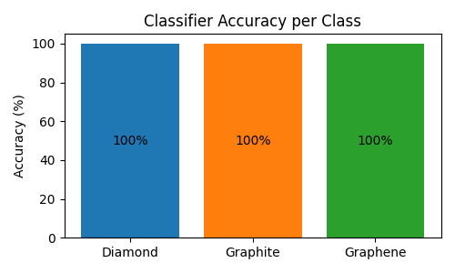
# Get predictions and compute per-class accuracy
class_names = ["Diamond", "Graphite", "Graphene"]
correct_per_class = {0: 0, 1: 0, 2: 0}
total_per_class = {0: 0, 1: 0, 2: 0}

for structure in structures:
    probabilities = (
        calc.run_model(
            structure,
            {"mtt::class_probabilities": ModelOutput(per_atom=False)},
        )["mtt::class_probabilities"]
        .block()
        .values.cpu()
        .squeeze(0)
        .numpy()
    )
    predicted_class = np.argmax(probabilities)
    # Get actual class from one-hot encoding
    actual_class = np.argmax(structure.info["class"])
    total_per_class[actual_class] += 1
    if predicted_class == actual_class:
        correct_per_class[actual_class] += 1

# Compute accuracy for each class
accuracies = [
    correct_per_class[i] / total_per_class[i] * 100 if total_per_class[i] > 0 else 0
    for i in range(3)
]

# Create a bar plot showing per-class accuracy
plt.figure(figsize=(5, 3))
bars = plt.bar(class_names, accuracies, color=["#1f77b4", "#ff7f0e", "#2ca02c"])
plt.ylabel("Accuracy (%)")
plt.title("Classifier Accuracy per Class")
plt.ylim(0, 105)

# Add value labels in the middle of bars
for bar, acc in zip(bars, accuracies, strict=True):
    plt.text(
        bar.get_x() + bar.get_width() / 2,
        bar.get_height() / 2,
        f"{acc:.0f}%",
        ha="center",
        va="center",
        fontsize=10,
    )

plt.tight_layout()
plt.show()

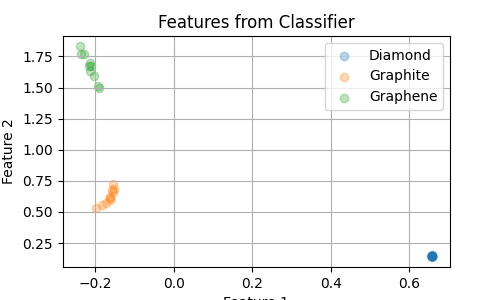
Now, we extract the features learned by the classifier in our “bottleneck” layer. Having only 2 dimensions allows us to easily visualize them. A low dimensionality is also necessary if we want to use these features as collective variables in enhanced sampling simulations. By default the last layer before the output is used as bottleneck, but this can be configured with the model hyperparameter feature_layer_index.

# Extract features
bottleneck_features = []
labels = []
probabilities_list = []
for structure in structures:
    features = (
        calc.run_model(
            structure,
            {"features": ModelOutput(per_atom=False)},
        )["features"]
        .block()
        .values.cpu()
        .squeeze(0)
        .numpy()
    )
    probs = (
        calc.run_model(
            structure,
            {"mtt::class_probabilities": ModelOutput(per_atom=False)},
        )["mtt::class_probabilities"]
        .block()
        .values.cpu()
        .squeeze(0)
        .numpy()
    )
    bottleneck_features.append(features)
    # Get class from one-hot encoding
    labels.append(np.argmax(structure.info["class"]))
    probabilities_list.append(probs)
bottleneck_features = np.array(bottleneck_features)
labels = np.array(labels)

# Plot the features for the three classes
plt.figure(figsize=(5, 3))
for class_id in np.unique(labels):
    mask = labels == class_id
    if class_id == 0:
        label = "Diamond"
    elif class_id == 1:
        label = "Graphite"
    else:
        label = "Graphene"
    plt.scatter(
        bottleneck_features[mask, 0],
        bottleneck_features[mask, 1],
        label=label,
        alpha=0.3,
    )
plt.xlabel("Feature 1")
plt.ylabel("Feature 2")
plt.title("Features from Classifier")
plt.legend()
plt.grid()
plt.show()

Interactive Visualization with Chemiscope

We can also create an interactive visualization using chemiscope, which allows us to explore the relationship between the structures and their bottleneck features.

# Prepare class labels as strings for visualization
class_names = ["Diamond", "Graphite", "Graphene"]
class_labels = [class_names[label] for label in labels]

# Prepare probabilities for all classes
probabilities_array = np.array(probabilities_list, dtype=np.float64)

# Create properties dictionary for chemiscope
properties = {
    "Feature 1": bottleneck_features[:, 0],
    "Feature 2": bottleneck_features[:, 1],
    "Class": class_labels,
    "Probability Diamond": probabilities_array[:, 0],
    "Probability Graphite": probabilities_array[:, 1],
    "Probability Graphene": probabilities_array[:, 2],
}

# Create the chemiscope visualization
chemiscope.show(
    structures,
    properties=properties,
    settings={
        "map": {
            "x": {"property": "Feature 1"},
            "y": {"property": "Feature 2"},
            "color": {"property": "Class"},
        },
        "structure": [{"unitCell": True}],
    },
)

×

Using the classifier model in PLUMED

The trained classifier model can also be used within PLUMED to define collective variables based on the features learned by the classifier. Instructions for using metatrain models with PLUMED can be found here.