Running Molecular Dynamics with ASE

This tutorial shows how to use metatensor atomistic models to run Molecular Dynamics (MD) simulation using ASE. ASE is not the only way to run MD with metatensor models, but it is very easy to setup and use.

from typing import Dict, List, Optional

# tools to run the simulation
import ase.build
import ase.md
import ase.md.velocitydistribution
import ase.units

# tools for visualization
import ase.visualize.plot
import chemiscope
import matplotlib.pyplot as plt

# the usuals suspects
import numpy as np
import torch

from metatensor.torch import Labels, TensorBlock, TensorMap
from metatensor.torch.atomistic import (
    MetatensorAtomisticModel,
    ModelCapabilities,
    ModelMetadata,
    ModelOutput,
    System,
)

# Integration with ASE calculator for metatensor atomistic models
from metatensor.torch.atomistic.ase_calculator import MetatensorCalculator

The energy model

To run simulations, we’ll need a model. For simplicity and keeping this tutorial short, we’ll use a model for Einstein’s solid, where all atoms oscillate around their equilibrium position as harmonic oscillators, but don’t interact with one another. The energy of each atoms is given by:

\[E_i = k * \left(\vec{r_i} - \vec{r_i}^0\right)^2,\]

where \(k\) is a harmonic force constant, \(\vec{r_i}\) the position of atom \(i\) and \(\vec{r_i}^0\) the position of atom \(i\) at equilibrium. The energy of the whole system is then

\[E = \sum_i E_i.\]

Let’s implement this model! You can check the Exporting a model tutorial for more information on how to define your own custom models.

class HarmonicModel(torch.nn.Module):
    def __init__(self, force_constant: float, equilibrium_positions: torch.Tensor):
        """Create an ``HarmonicModel``.

        :param force_constant: force constant, in ``energy unit / (length unit)^2``
        :param equilibrium_positions: torch tensor with shape ``n x 3``, containing the
            equilibrium positions of all atoms
        """
        super().__init__()
        assert force_constant > 0
        self.force_constant = force_constant
        self.equilibrium_positions = equilibrium_positions

    def forward(
        self,
        systems: List[System],
        outputs: Dict[str, ModelOutput],
        selected_atoms: Optional[Labels],
    ) -> Dict[str, TensorMap]:
        if list(outputs.keys()) != ["energy"]:
            raise ValueError(
                "this model can only compute 'energy', but `outputs` contains other "
                f"keys: {', '.join(outputs.keys())}"
            )

        # we don't want to worry about selected_atoms yet
        if selected_atoms is not None:
            raise NotImplementedError("selected_atoms is not implemented")

        if outputs["energy"].per_atom:
            raise NotImplementedError("per atom energy is not implemented")

        # compute the energy for each system by adding together the energy for each atom
        energy = torch.zeros((len(systems), 1), dtype=systems[0].positions.dtype)
        for i, system in enumerate(systems):
            assert len(system) == self.equilibrium_positions.shape[0]
            r0 = self.equilibrium_positions
            energy[i] += torch.sum(self.force_constant * (system.positions - r0) ** 2)

        # add metadata to the output
        block = TensorBlock(
            values=energy,
            samples=Labels("system", torch.arange(len(systems)).reshape(-1, 1)),
            components=[],
            properties=Labels("energy", torch.tensor([[0]])),
        )
        return {
            "energy": TensorMap(keys=Labels("_", torch.tensor([[0]])), blocks=[block])
        }

Initial simulation state

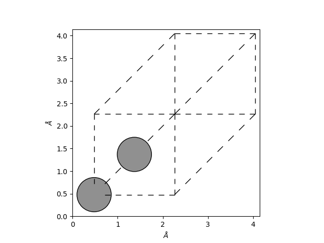
Now that we have a model for the energy of our system, let’s create some initial simulation state. We’ll build a 3x3x3 super cell of diamond carbon. In practice, you could also read the initial state from a file using ase.io.read().

primitive = ase.build.bulk(name="C", crystalstructure="diamond", a=3.567)

ax = ase.visualize.plot.plot_atoms(primitive, radii=0.5)
ax.set_xlabel("$\\AA$")
ax.set_ylabel("$\\AA$")
plt.show()

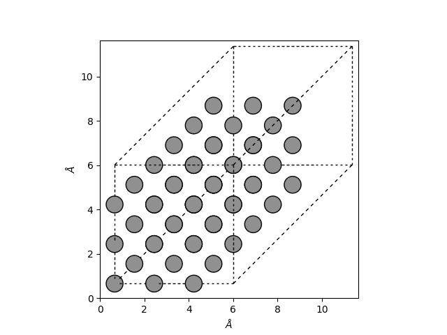
And now let’s make a super cell with this

atoms = ase.build.make_supercell(primitive, 3 * np.eye(3))

ax = ase.visualize.plot.plot_atoms(atoms, radii=0.5)
ax.set_xlabel("$\\AA$")
ax.set_ylabel("$\\AA$")

plt.show()

We’ll also need to initialize the velocities of the atoms to match our simulation temperature.

# The atoms start with zero velocities, hence zero kinetic energy and zero temperature
print("before:")
print("kinetic energy =", atoms.get_kinetic_energy(), "eV")
print("temperature =", atoms.get_temperature(), "K")

ase.md.velocitydistribution.MaxwellBoltzmannDistribution(atoms, temperature_K=300)
print("\nafter:")
print("kinetic energy =", atoms.get_kinetic_energy(), "eV")
print("temperature =", atoms.get_temperature(), "K")

before:
kinetic energy = 0.0 eV
temperature = 0.0 K

after:
kinetic energy = 1.8574322169102175 eV
temperature = 266.1063350226441 K

Running the simulation

The final step to run the simulation is to register our model as the energy calculator for these atoms. This is the job of ase_calculator.MetatensorCalculator, which takes either an instance of MetatensorAtomisticModel or the path to a pre-exported model, and allow to use it to compute the energy, forces and stress acting on a system.

# define & wrap the model, using the initial positions as equilibrium positions
model = HarmonicModel(
    force_constant=3.14159265358979323846,
    equilibrium_positions=torch.tensor(atoms.positions),
)

capabilities = ModelCapabilities(
    outputs={
        "energy": ModelOutput(quantity="energy", unit="eV", per_atom=False),
    },
    atomic_types=[6],
    interaction_range=0.0,
    length_unit="Angstrom",
    supported_devices=["cpu"],
    dtype="float32",
)

# we don't want to bother with model metadata, so we define it as empty
metadata = ModelMetadata()
wrapper = MetatensorAtomisticModel(model.eval(), metadata, capabilities)

# Use the wrapped model as the calculator for these atoms
atoms.calc = MetatensorCalculator(wrapper)

We’ll run the simulation in the constant volume/temperature thermodynamics ensemble (NVT or Canonical ensemble), using a Langevin thermostat for time integration. Please refer to the corresponding documentation (ase.md.langevin.Langevin) for more information!

integrator = ase.md.Langevin(
    atoms,
    timestep=1.0 * ase.units.fs,
    temperature_K=300,
    friction=0.1 / ase.units.fs,
)

# collect some data during the simulation
trajectory = []
potential_energy = []
kinetic_energy = []
total_energy = []
temperature = []

for step in range(800):
    # run a single simulation step
    integrator.run(1)

    # collect data about the simulation
    potential_energy.append(atoms.get_potential_energy())
    kinetic_energy.append(atoms.get_kinetic_energy())
    total_energy.append(atoms.get_total_energy())
    temperature.append(atoms.get_temperature())

    if step % 10 == 0:
        trajectory.append(atoms.copy())

We can use chemiscope to visualize the trajectory

viewer_settings = {"bonds": False, "playbackDelay": 70}
chemiscope.show(trajectory, mode="structure", settings={"structure": [viewer_settings]})

×

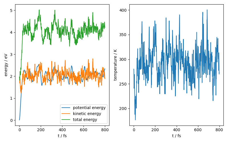
We can also look at the time evolution of some physical constants for our system:

fig, ax = plt.subplots(1, 2, figsize=(8, 5))

ax[0].plot(range(800), potential_energy, label="potential energy")
ax[0].plot(range(800), kinetic_energy, label="kinetic energy")
ax[0].plot(range(800), total_energy, label="total energy")
ax[0].legend()
ax[0].set_xlabel("t / fs")
ax[0].set_ylabel("energy / eV")

ax[1].plot(range(800), temperature)
ax[1].set_xlabel("t / fs")
ax[1].set_ylabel("temperature / K")

fig.tight_layout()
fig.show()

Using a pre-exported model

As already mentioned, ase_calculator.MetatensorCalculator also work with a pre-exported model, meaning you can also run simulations without defining or re-training a model:

wrapper.save("exported-model.pt")

atoms.calc = MetatensorCalculator("exported-model.pt")

print(atoms.get_potential_energy())
integrator.run(10)

1.9017589092254639

True