Creating models that use neighbor lists

This tutorial demonstrates how to create an atomistic model that requires a neighbor list, and use it to run MD simulations. This tutorial assumes knowledge of how to export an atomistic model and run it with the ASE calculator. If you haven’t read the corresponding examples, please refer to Exporting a model and Running Molecular Dynamics with ASE.

As depicted below, one or more neighbor lists will be requested by the model, computed by the simulation engine and attached to the Systems. The Systems with the neighbor list is then passed to the model.

The simulation engine computes the neighbor lists for the model, which then uses them to predict outputs. This figure is a subset of the figure in Data flow between the model and engine.

As example, we will run a 1 ps short molecular dynamics simulation of 125 already equilibrated liquid argon atoms interacting via Lennard-Jones within a cutoff of 5 Å. The system will be simulated at a temperature of 94.4 K and a mass density of 1.374 g/cm³. In the end, we will obtain the pair-correlation function \(g(r)\) of the liquid.

from typing import Dict, List, Optional

# tools for analysis
import ase.geometry.rdf

# tools to run the simulation and visualization
import ase.io
import ase.md
import ase.neighborlist
import ase.visualize.plot
import chemiscope
import matplotlib.pyplot as plt

# the usual suspects
import numpy as np
import torch

from metatensor.torch import Labels, TensorBlock, TensorMap
from metatensor.torch.atomistic import (
    MetatensorAtomisticModel,
    ModelCapabilities,
    ModelMetadata,
    ModelOutput,
    NeighborListOptions,
    System,
)

# Integration with ASE calculator for metatensor atomistic models
from metatensor.torch.atomistic.ase_calculator import MetatensorCalculator

The simulation system

We load the pre-equilibrated liquid argon system from a file.

atoms = ase.io.read("liquid-argon.xyz")

The system was generated based on a 5x5x5 supercell of a simple cubic (sc) cell with a lattice constant of a = 3.641 Å. After initialization of the velocities, the system was run for 100 ps with the same parameters we will use below and the final state can be visualized as

ax = ase.visualize.plot.plot_atoms(atoms, radii=0.5)
ax.set_xlabel("$\\AA$")
ax.set_ylabel("$\\AA$")
plt.show()

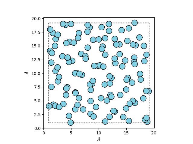
The system already has velocities and the expected density of 1.374 g/cm³.

u_to_g = 1.66053906660e-24
Å_to_cm = 1e-08

mass_density = sum(atoms.get_masses()) / atoms.cell.volume * u_to_g / Å_to_cm**3

print(f"ρ_m = {mass_density:.3f} g/cm³")

ρ_m = 1.374 g/cm³

Metatensor’s neighbor lists

Note

The steps below of creating a neighbor list, wrapping it inside a TensorBlock and attaching it to a system will be done by the simulation engine and must not be handled by the model developer. How to request a neighbor list will be presented below when the actual model is defined.

Before implementing the actual model, let’s take a look at how metatensor stores neighbor lists inside a System object. We start by computing the neighbor list for our argon systen using ASE.

i, j, S, D = ase.neighborlist.neighbor_list(quantities="ijSD", a=atoms, cutoff=5.0)

The ase.neighborlist.neighbor_list() function returns the neighbor indices: quantities "i" and "j", the neighbor shifts "S", and the distance vectors "D". We now stack these together and convert them into the suitable types.

i = torch.from_numpy(i.astype(int))
j = torch.from_numpy(j.astype(int))
neighbor_indices = torch.stack([i, j], dim=1)
neighbor_shifts = torch.from_numpy(S.astype(int))

print("neighbor_indices:", neighbor_indices)
print("neighbor_shifts:", neighbor_shifts)

neighbor_indices: tensor([[  0,   6],
        [  0,   1],
        [  0,  20],
        ...,
        [124, 104],
        [124,  78],
        [124,  98]])
neighbor_shifts: tensor([[ 1,  0,  0],
        [ 0,  0,  0],
        [ 1, -1, -1],
        ...,
        [ 0,  0,  0],
        [ 0,  0,  0],
        [ 0,  0,  0]])

Creating a neighbor list

We now assemble the neighbor list following metatensor conventions. First, we create the samples metadata for the TensorBlock which will hold the neighbor list.

sample_values = torch.hstack([neighbor_indices, neighbor_shifts])
samples = Labels(
    names=[
        "first_atom",
        "second_atom",
        "cell_shift_a",
        "cell_shift_b",
        "cell_shift_c",
    ],
    values=sample_values,
)

neighbors = TensorBlock(
    values=torch.from_numpy(D).reshape(-1, 3, 1),
    samples=samples,
    components=[Labels.range("xyz", 3)],
    properties=Labels.range("distance", 1),
)

print(neighbors)

TensorBlock
    samples (1356): ['first_atom', 'second_atom', 'cell_shift_a', 'cell_shift_b', 'cell_shift_c']
    components (3): ['xyz']
    properties (1): ['distance']
    gradients: None

The data and metadata inside the neighbors object do not contain information about the cutoff and whether this is a full or half neighbor list. To account for this, metatensor neighbor lists are always stored together with NeighborListOptions. For our system, these options can be saved as

options = NeighborListOptions(cutoff=5.0, full_list=True)

We set full_list=True because ASE computes a “full” list (as opposed to a half list) where each i, j pair appears twice, stored once as i, j and once as j, i.

Now we can, in principle, attach the neighbor list to a metatensor system using

system.add_neighbor_list(options=options, neighbors=neighbors)

Accessing data in neighbor lists

Now that we have a neighbor list, we can access the data and metadata. First, we can extract the distances vectors between the neighboring pairs within the cutoff, which we can then use in our models.

distances = neighbors.values

print(distances.shape)

torch.Size([1356, 3, 1])

We can also get the metadata values like neighbor indices or the neighbor shifts using the Labels.column and Labels.view methods.

i = neighbors.samples.column("first_atom")
j = neighbors.samples.column("second_atom")

neighbor_indices = neighbors.samples.view(["first_atom", "second_atom"]).values
neighbor_shifts = neighbors.samples.view(
    ["cell_shift_a", "cell_shift_b", "cell_shift_c"]
).values

As mentioned above, in practical use cases you will not have to compute neighbor lists yourself, but instead the simulation engine will compute it for you and you’ll just need to get the right list for a given System using the corresponding options:

neighbors = system.get_neighbor_list(options)

You can also loop over all attached lists of a System using System.known_neighbor_lists() to find a suitable one based on NeighborListOptions attributes like cutoff, full_list, and requestors.

A Lennard-Jones model

Now that we know how the neighbor data is stored and can be accessed, and know how to use it we can construct our Lennard-Jones model with a fixed cutoff. The Lennard-Jones potential is a mathematical basis to approximate the interaction between a pair of neutral atoms or molecules. It is given by the equation:

\[V(r) = 4\epsilon \left[ \left( \frac{\sigma}{r} \right)^{12} - \left( \frac{\sigma}{r} \right)^{6} \right]\]

where \(\epsilon\) is the depth of the potential well, \(\sigma\) is the finite distance at which the inter-particle potential is zero, and \(r\) is the distance between the particles. The 12-6 form is chosen because the \(r^{12}\) term approximates the Pauli repulsion at short ranges, while the \(r^6\) term represents the attractive van der Waals forces. The \(r^{12}\) is chosen because it is just the square of the \(r^6\) and therefore allows fast evaluation.

A Lennard-Jones potential is well-suited for argon because it accurately represents the van der Waals forces that dominate the interactions between argon atoms, as for all noble gases. This potential was used in one of the first MD simulations: “Correlation in the motions of atoms in liquid Argon” by A. Rahman (Phys. Rev. 136, A405-A411, 1964), which demonstrated the effectiveness of continuous potentials in molecular dynamics.

The model below is a simplified version of a more complex Lennard-Jones model. The linked version also implements per_atom energies as well as atom selection using the selected_atoms parameter of the forward() method. In this model, we shift the energy by its value at the cutoff. This will break the conservativeness of the potential, which is unproblematic in here because we use a large cutoff and therefore the potential already almost decayed to zero. For more sophisticated methods like a polynomial switching potential like XPLOR, we refer to the literature.

class LennardJonesModel(torch.nn.Module):
    """Implementation of a single particle type Lennard-Jones potential."""

    def __init__(self, cutoff, sigma, epsilon):
        super().__init__()

        # define neighbor list options to request the right set of neighbors
        self._nl_options = NeighborListOptions(cutoff=cutoff, full_list=False)

        self._sigma = sigma
        self._epsilon = epsilon

        # shift the energy to 0 at the cutoff
        self._shift = 4 * epsilon * ((sigma / cutoff) ** 12 - (sigma / cutoff) ** 6)

    def requested_neighbor_lists(self) -> List[NeighborListOptions]:
        """Method declaring which neighbors lists this model desires.

        The method is required to tell an simulation engine (here ase) to compute and
        attach the requested neighbor list to a system which will be passed to the
        ``forward`` method defined below

        Note that a model can request as many neighbor lists as it wants
        """
        return [self._nl_options]

    def forward(
        self,
        systems: List[System],
        outputs: Dict[str, ModelOutput],
        selected_atoms: Optional[Labels],
    ) -> Dict[str, TensorMap]:
        if list(outputs.keys()) != ["energy"]:
            raise ValueError(
                "this model can only compute 'energy', but `outputs` contains other "
                f"keys: {', '.join(outputs.keys())}"
            )

        # we don't want to worry about selected_atoms yet
        if selected_atoms is not None:
            raise NotImplementedError("selected_atoms is not implemented")

        if outputs["energy"].per_atom:
            raise NotImplementedError("per atom energy is not implemented")

        # Initialize device so we can access it outside of the for loop
        device = torch.device("cpu")
        for system in systems:
            device = system.device
            neighbors = system.get_neighbor_list(self._nl_options)
            distances = neighbors.values.reshape(-1, 3)

            sigma_r_6 = (self._sigma / torch.linalg.vector_norm(distances, dim=1)) ** 6
            sigma_r_12 = sigma_r_6 * sigma_r_6
            e = 4.0 * self._epsilon * (sigma_r_12 - sigma_r_6) - self._shift

        samples = Labels(
            ["system"], torch.arange(len(systems), device=device).reshape(-1, 1)
        )

        block = TensorBlock(
            values=torch.sum(e).reshape(-1, 1),
            samples=samples,
            components=torch.jit.annotate(List[Labels], []),
            properties=Labels(["energy"], torch.tensor([[0]], device=device)),
        )
        return {
            "energy": TensorMap(
                Labels("_", torch.tensor([[0]], device=device)), [block]
            ),
        }

In the model above, in addition to the required __init__() and ModelInterface.forward() methods, we also implemented the ModelInterface.requested_neighbor_lists() method, which declares the neighbor list our model requires.

Running the simulation

We now define and wrap the model, using the initial positions and the Lennard-Jones parameters taken from Méndez-Bermúdez et.al, Phys. Commun. 2022.

Note

The units of the Lennard Jones parameters from the reference are in "Angstrom" and "kJ/mol". We declare the (energy) unit and length_unit accordiningly when defining the ModelCapabilities object below. From then on, metatensor is taking care of the correct unit conversion when the energies and forces are passed to the simulation engine.

sigma = 3.3646  # Å
epsilon = 0.94191  # kJ / mol

model = LennardJonesModel(
    cutoff=5.0,
    sigma=sigma,
    epsilon=epsilon,
)

capabilities = ModelCapabilities(
    outputs={
        "energy": ModelOutput(quantity="energy", unit="kJ/mol", per_atom=False),
    },
    atomic_types=[18],
    interaction_range=5.0,
    length_unit="Angstrom",
    supported_devices=["cpu"],
    dtype="float32",
)

wrapper = MetatensorAtomisticModel(model.eval(), ModelMetadata(), capabilities)

# Use the wrapped model as the calculator for these atoms
atoms.calc = MetatensorCalculator(wrapper)

We’ll run the simulation in the constant volume/temperature thermodynamic ensemble (NVT or Canonical ensemble), using a Langevin thermostat for time integration. Please refer to the corresponding documentation (ase.md.langevin.Langevin) for more information!

integrator = ase.md.Langevin(
    atoms,
    timestep=2.0 * ase.units.fs,
    temperature_K=94.4,
    friction=0.1 / ase.units.fs,
)

trajectory = []

for _ in range(50):
    # run a single simulation for 10 steps
    integrator.run(10)

    # collect data about the simulation
    trajectory.append(atoms.copy())

We can use chemiscope to visualize the trajectory

viewer_settings = {"bonds": False, "playbackDelay": 70}
chemiscope.show(trajectory, mode="structure", settings={"structure": [viewer_settings]})

×

We finally compute and plot the avaregae pair-correlation function \(g(r)\) of the recorded trajectory.

rdf = []
for atoms in trajectory:
    rdf_step, rdf_dists = ase.geometry.rdf.get_rdf(atoms, rmax=9.0, nbins=100)
    rdf.append(rdf_step)

fig, ax = plt.subplots()

ax.plot(rdf_dists, np.mean(rdf, axis=0))

ax.set_xlabel("distance / Å")
ax.set_ylabel("$g(r)$")
ax.minorticks_on()

fig.tight_layout()
fig.show()

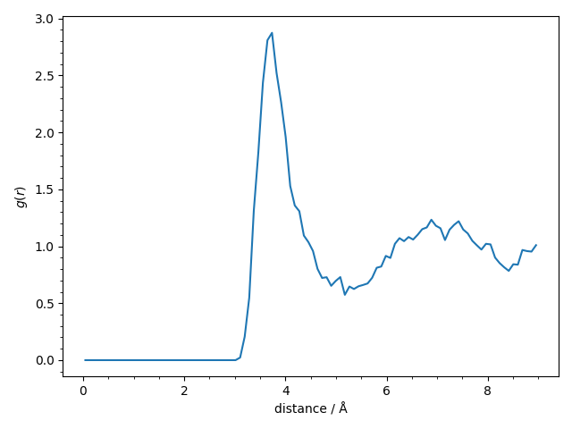
The pair-correlation function shows the usual structure for a liquid and we find the expected first narrow peak at 3.7 Å and a second broader peak at 7.0 Å.